Execution model

Introduction

Pine Script® relies on an event-driven, sequential execution model to control how a script’s compiled source code runs in charts, alerts, Deep Backtesting mode, and the Pine Screener.

In contrast to the traditional execution model of most programming languages, Pine’s runtime system executes a script repeatedly on the sequence of historical bars and realtime ticks in the dataset on which it runs, performing separate calculations for each bar as it progresses. After each execution on a closed bar, the necessary data from that execution becomes part of an internal time series, and the script can use that data in its calculations on subsequent bars.

This combination of sequential executions and storage enables programmers to use minimal code to write scripts with dynamic calculations that advance across a dataset bar by bar.

The execution model and time series structure closely connect to the type system — together, they define how a script behaves as it runs on a dataset. Although it’s possible to write simple scripts without understanding these foundational topics, learning about them and their nuances is key to becoming proficient in Pine Script.

This page explains the execution model in two parts: The basics and The details. The first part provides quick, actionable information about the model for beginners. The second part offers an advanced, in-depth breakdown of the model’s workings and unique behaviors. To make the most of the information on this page, we recommend that newcomers to Pine Script start with The basics, learn about other topics in this manual, and then come back to this page for the advanced details.

The basics

The following sections outline core principles of the execution model for beginners. If you are new to Pine Script, start here.

Bar-by-bar execution

The dataset for a symbol on a given timeframe, as shown on a chart, consists of a sequence of bars representing a time series. Each bar in the sequence represents the price and volume for a specific time period. The first (leftmost) bar on a chart corresponds to the earliest period, and the last (rightmost) bar corresponds to the most recent period.

Much of the power of Pine Script stems from its ability to process this time series data efficiently. When a user runs a script, its code does not execute just once; it executes from start to end on each bar in the symbol’s dataset individually, progressing from the first available bar to the most recent bar. Each separate script execution performs calculations or generates outputs (e.g., plots) for a specific bar using the data available on that bar.

A script can retrieve price, volume, and other essential data for each bar on which it executes by using the built-in variables that hold bar information, such as open, high, low, close, and volume. These variables automatically update before each new execution to store the values for the current bar.

For example, the simple script below uses the plot() function to display the series of close values (i.e., the closing price of each bar) on the chart:

When a user first adds this script to their chart, its code executes once for every bar in the available dataset. As the script runs on the data, two primary steps occur on each bar:

1. The close variable automatically updates to hold the current bar’s latest price.
2. The plot() function call plots the updated close value at the current bar’s position.

When the script finishes its run from the first bar to the most recent bar, the result is a simple line plot showing the progression of closing prices across the chart’s history:

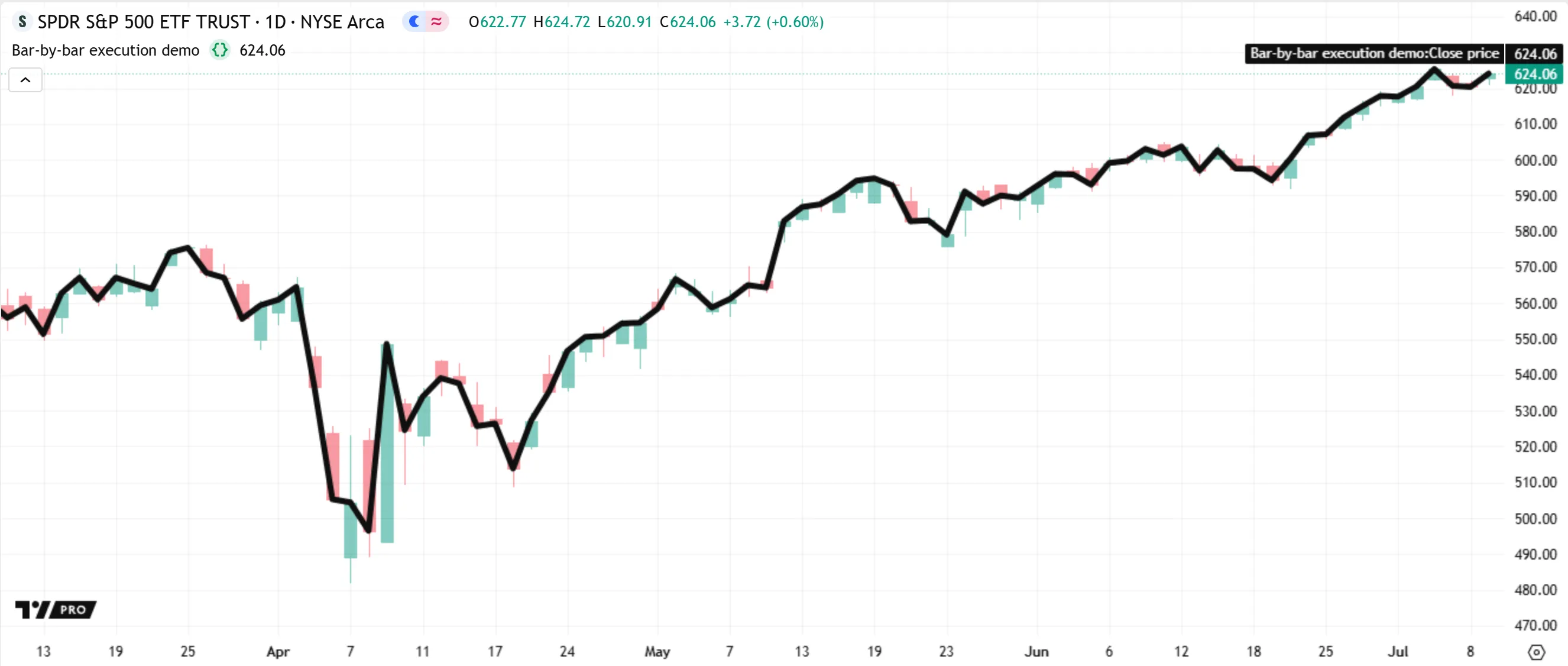
Note that the above script evaluates the plot() function call once for every bar on the chart, not just once in total. On each separate execution, the call defines the plotted point for the current bar: the chart’s first bar during the first execution, the second bar during the next, and so on.

This pattern illustrates a key principle of Pine’s execution model: on each successive execution, a script re-evaluates function calls and other expressions within its required scopes to perform separate calculations for the current bar.

Repeated code evaluation also applies to variable declarations. By default, a script does not declare a variable only once throughout its runtime; the script re-declares that variable and assigns an initial value based on the current bar’s data during each new evaluation of its scope.

Let’s look at a simple example. The following script declares an x variable of the “int” type with an initial value of 0. Then, it increases the variable’s value by 10 with the addition assignment operator (+=). The script calls plot() to display the value of x on each bar in a separate pane:

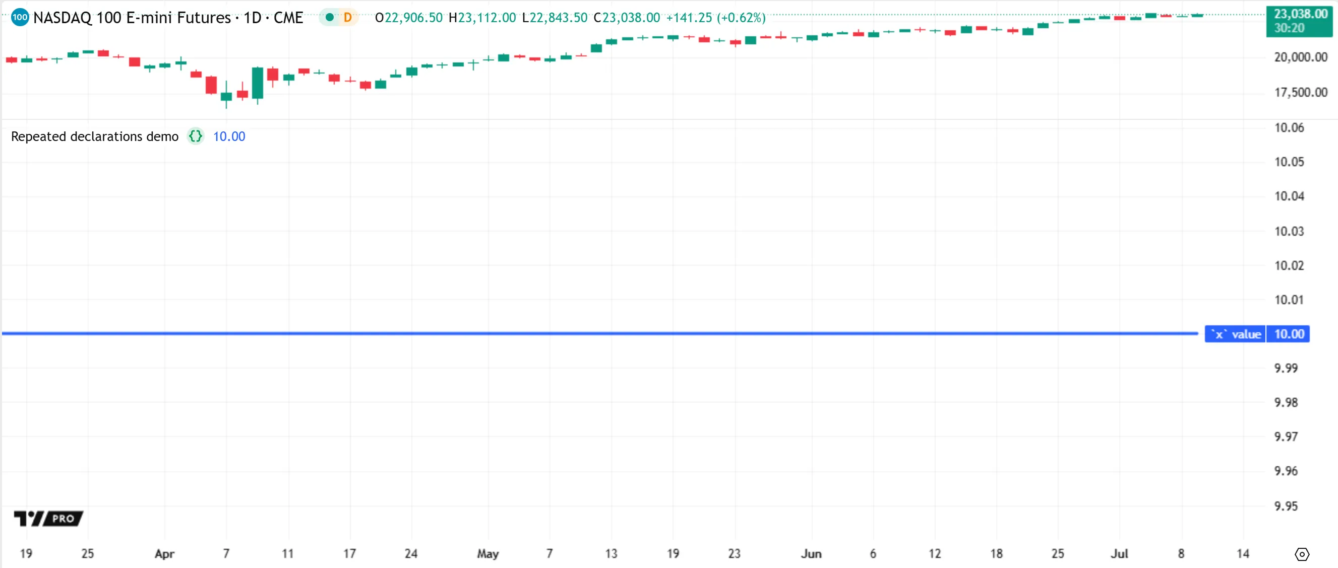
As shown above, the script plots a value of 10 on every bar, because the x variable does not carry over from bar to bar; the script declares the variable repeatedly. On each bar, the script re-declares x with an initial value of 0, then adds 10 to that value, resulting in a final value of 10 for every plotted point.

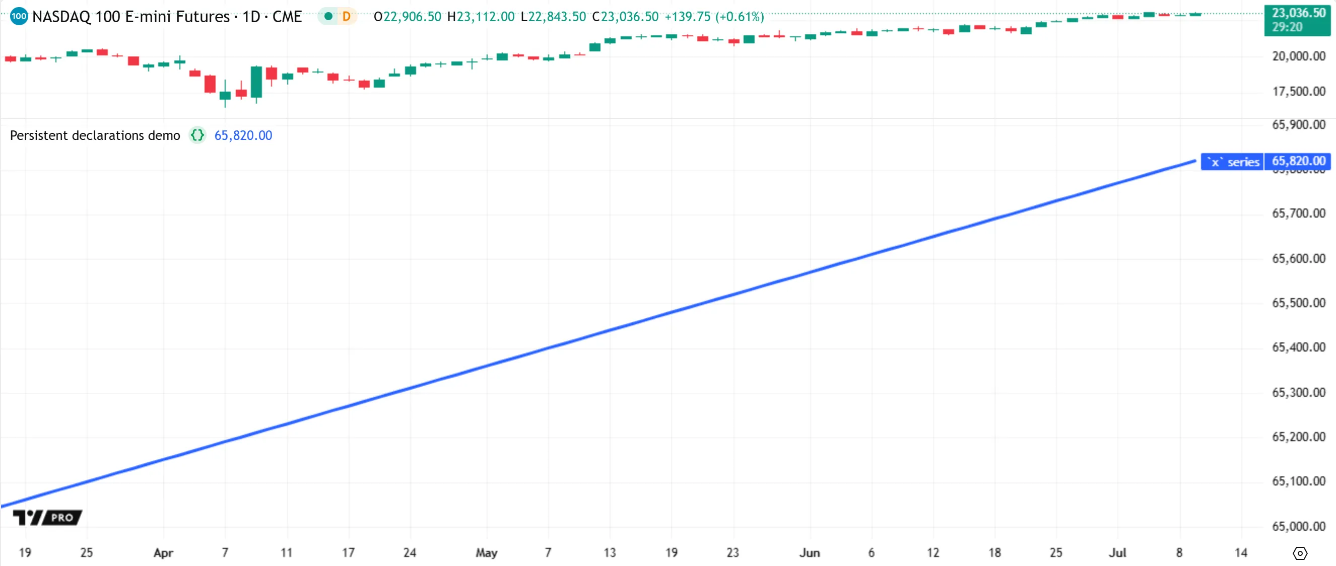
Programmers can change the behavior of a variable, enabling it to persist and preserve updates to its value across bars, by including the var keyword in its declaration, as described in the Declaration modes section of the Variable declarations page.

Below, we modify the previous script by adding var to the x declaration. Now, the script declares and initializes x only once — on the first bar — and that variable persists across all bars that follow. The script now plots a line that increases by 10 on each bar, because x preserves the result from each addition across the chart’s history. The value changes from 0 to 10 on the first bar, then to 20 on the second, and so on:

Storing and using data from previous bars

As a script runs on a dataset, the states of its variables, function calls, and other expressions are automatically committed (saved) to an internal time series on each bar, creating historical trails of previous bar values that the script can access during its calculations on the current bar. The script can use these previous values by doing either of the following:

• Using the [] history-referencing operator. The number in the square brackets represents how many bars back from the current bar the script looks to retrieve a past value. For instance, close[1] retrieves the close value from one bar before the current bar, and close[100] retrieves the value from 100 bars back.
• Calling the built-in functions that calculate on past values internally, such as ta.*() functions. For instance, ta.change(close, 10) calculates the difference between the current value of close and its value from 10 bars back.

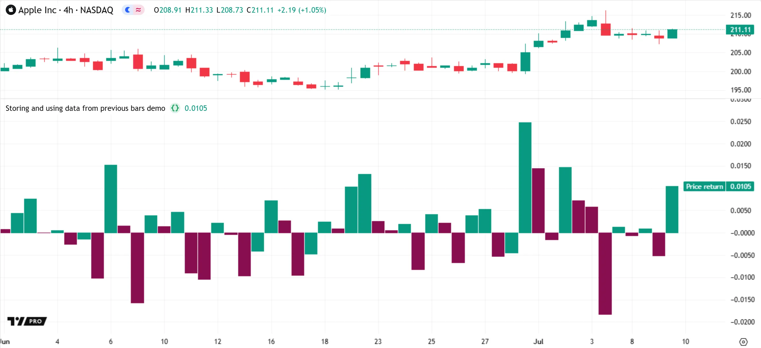
The example below uses both of the above techniques to perform calculations based on data from previous bars. The script calculates a series of bar-by-bar price returns and plots the result as color-coded columns. It declares two global variables on each bar: priceReturn for the calculated returns, and returnColor for the plot’s color. The priceReturn value is the result of dividing the current one-bar change in closing prices (ta.change(close, 1)) by the previous bar’s closing price (close[1]). The returnColor value is color.teal if the current value of priceReturn is higher than the value from the previous bar (priceReturn[1]), and color.maroon otherwise:

Note that:

• This script does not plot a column on bar 0 (the first bar). The priceReturn value is na on that bar, because there is no previous bar available for the script to reference at that point.

Realtime bars

When a script first runs on a chart, all closed bars in the accessed dataset are historical bars. These bars represent data for elapsed time periods where the final price and volume are confirmed. All indicators execute once per historical bar.

When the rightmost bar on the chart is open, it is a realtime bar. Unlike a historical bar, whose values are final, a realtime bar updates its values as new price or volume data becomes available. After the bar closes, it becomes an elapsed realtime bar, which is then no longer subject to change as the script runs.

Because the final values for a realtime bar are unknown until the bar closes, an indicator executes differently on that bar than it does on historical bars. The script executes not once, but repeatedly on the realtime bar — once for each new update (tick) — to recalculate its results using the latest data.

Before each recalculation on the realtime bar, the data for a script’s variables, expressions, and outputs on that bar is cleared, or reset. We refer to this process as rollback. The purpose of rollback is to revert the script to the same confirmed state it had when the realtime bar opened. This process ensures that the script’s calculations for the bar operate only on the latest available data, without relying on temporary data from the bar’s previous ticks.

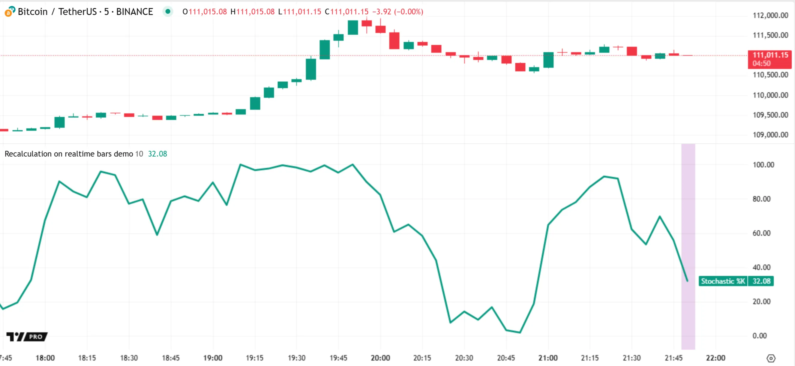
Let’s look at rollback and recalculation in action. The following script uses ta.stoch() to calculate the Stochastic oscillator based on the close, high, and low values over a specified number of bars, then plots the result in a separate pane. It also calls bgcolor() to highlight the background on each realtime bar — where barstate.isrealtime is true — for visual reference:

When we add the script to our chart, it executes once per bar in the chart’s history, from the leftmost bar to the rightmost bar. However, the rightmost bar on our chart is still open. Therefore, it is a realtime bar, not a historical bar. After the script reaches that bar, it begins executing once for every new update to the bar’s data. Each new script execution calculates on the latest available prices and replaces the bar’s previous result.

For instance, in the initial image below, the oscillator’s value 10 seconds into the open realtime bar (the one with the purple background) is 32.08:

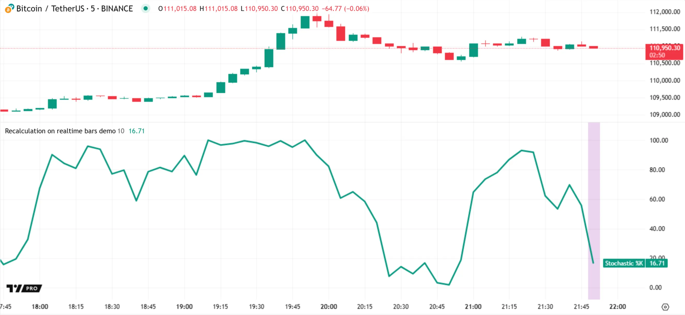
Every time the bar updates, rollback resets the script’s data for that bar, and the script recalculates its result using the latest high, low, and close values. Here, halfway through the realtime bar’s period, the oscillator’s plot now shows a value of 16.71:

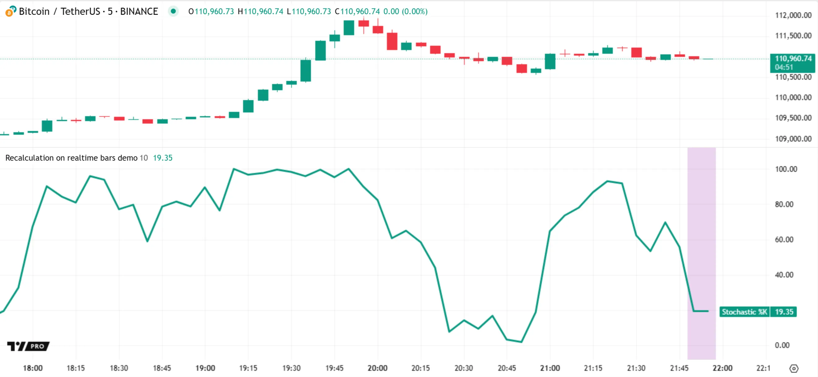
Recalculation continues for each successive update to the bar. Then, the script reaches the bar’s closing tick, where the prices become confirmed. On that tick, the script calculates the oscillator’s final value of 19.35. Afterward, another realtime bar opens, and the pattern of rollback and recalculation continues on that bar:

Note that:

• Only the values for a realtime bar’s final tick become part of the internal time series. The values from ticks before the bar’s close are not saved.
• The input.int() function returns a value of the “input int” qualified type. Values qualified as “input” are established before the first script execution, and they remain consistent throughout the script’s runtime. If the user changes the “Length” input to a new value, the script restarts to perform new calculations across the dataset using that value. See the Inputs page and the Qualifiers section of the Type system page to learn more about script inputs and the “input” qualifier.
• If the script restarts, all the realtime bars from the previous script run become historical bars in the new run. Therefore, after restarting, the script executes only once on each of those bars and does not highlight their background.

The details

The following sections provide in-depth details about Pine’s execution model, including the mechanics of executions on historical bars and realtime bars, which events trigger script executions, and how the runtime system maintains data across executions in a time series format.

Executions on historical bars

When a script loads on the chart or in another location after an execution-triggering event, its compiled source code executes on every accessible bar in the current dataset in order, starting with the first bar.

While the script loads, the runtime system performs the following steps for each bar that it accesses:

1. It updates the built-in variables that hold bar information. For instance, the system sets the open, high, low, and close variables to hold the OHLC price values of the bar before each execution.
2. It executes the script’s compiled code from start to end using the data available as of the current bar.
3. After the execution ends, the system commits (saves) all necessary data for the current bar to the time series. The script can then access that data from historical buffers during its executions on subsequent bars by using the history-referencing operator or the built-in functions that reference past bars internally.

These steps repeat for every successive bar up to the most recent bar. After the runtime system completes this process across the dataset, the script’s committed outputs — such as plots, drawings, Pine Logs, and Strategy Tester results — become available to the user.

All the closed bars on which the script executes while loading are historical, because they represent data points that were confirmed before the event that triggered the loading process. By default, all scripts execute once for each historical bar.

Let’s examine a simple indicator to understand how script executions work on historical bars.

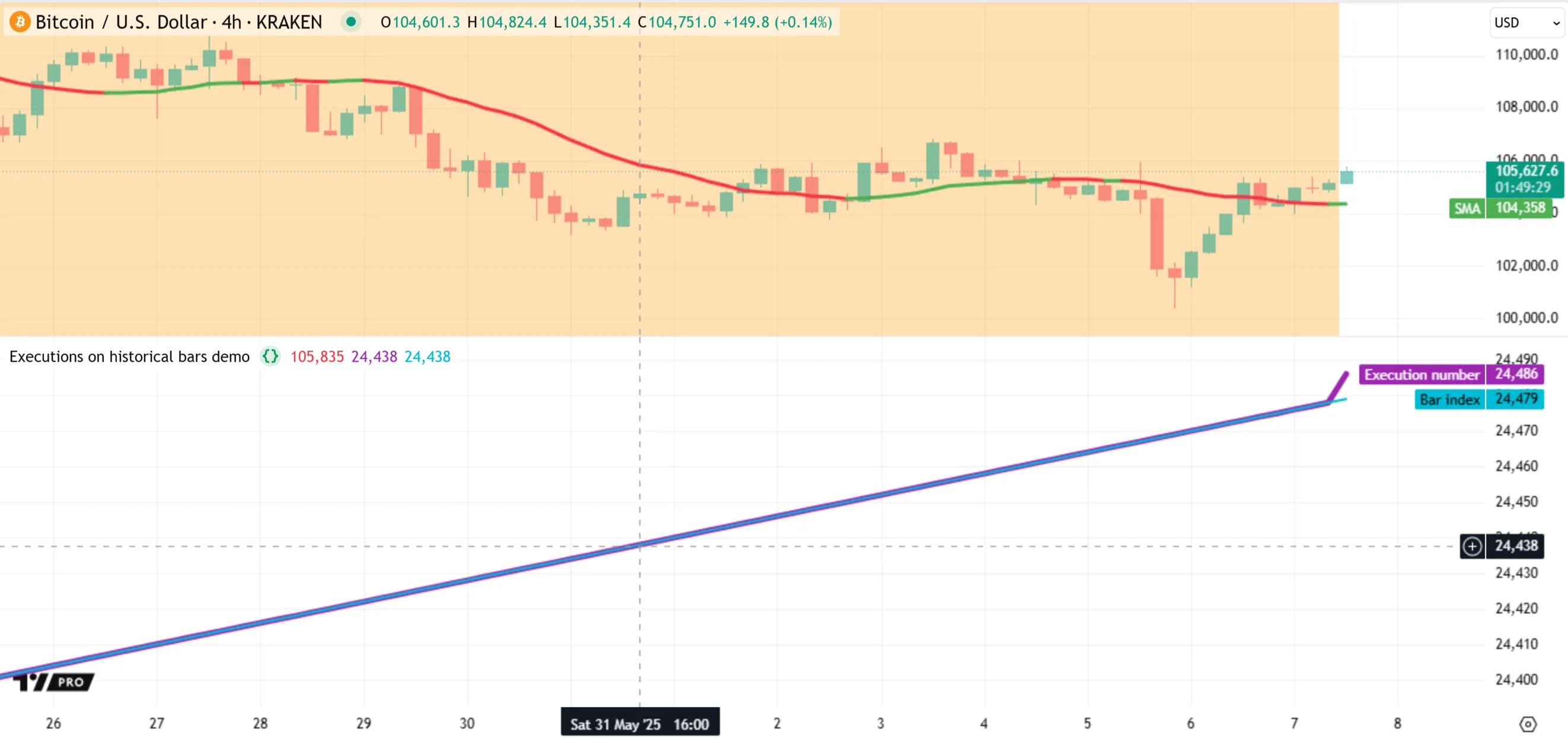
The script below calculates the 20-bar moving average of close values and plots the result on the chart. The color of the plot depends on whether the average is above or below the value on the previous bar. The script also increments an executionNum variable to count code executions, then plots the result alongside bar_index for comparison. Additionally, it highlights the background of historical bars in orange for visual reference:

The statements and expressions in this source code might appear static at first glance. However, they have dynamic behavior across bars because the system executes the script repeatedly — once for each successive data point. Below, we inspect the code step by step to explain how the script works during its historical executions.

The indicator() call at the top of the code is a declaration statement that defines the script’s type and properties once, at compile time. This statement does not execute as the script runs on the dataset:

Before each script execution on a bar, the runtime system updates the built-in bar_index and close variables required in the calculations. The bar_index value is the bar’s global time series index, where 0 represents the first bar, 1 represents the second, and so on. The close variable holds the bar’s latest price. For historical bars, its value is the final price at the bar’s closing time.

Each time that the script executes, it declares and initializes a global sma variable of the “float” type. This variable declaration happens on every execution because the code line does not specify a declaration mode. The variable’s assigned value is the result of a ta.sma() function call. The call returns the average of the latest 20 close values as of the current bar, or na if fewer than 20 bars are available. After the execution ends, the system commits the new value of sma to the time series:

Note that:

• The //@variable comment above the sma declaration is an annotation that documents the variable in the code. The Pine Editor displays the comment in a pop-up window when the user hovers the mouse pointer over the variable.

During each execution, the script also initializes a plotColor variable of the “color” type. The script uses a ternary operation that compares the current sma value to sma[1] — the last committed value for sma as of the previous bar — to determine the plotColor variable’s assigned value. If the current sma value is higher than the last committed value, the plotColor value is color.green. Otherwise, it is color.red:

In contrast to the variables above, the script does not initialize the executionNum variable on every execution. Instead, initialization happens only once — on the first bar — because the variable declaration is in the global scope and uses the varip keyword. Once initialized, the variable persists across all subsequent bars and the ticks within those bars. Only the reassignment or compound assignment operators can change its value:

The code following the executionNum declaration uses the addition assignment operator (+=) to increase the variable’s value by one on each new execution. Starting from -1, the value increases to 0 on the first execution after initialization, then 1 on the second, and so on:

The script evaluates the plot() and bgcolor() calls on every execution. Each plot() call creates a new point on a line plot at the bar’s location on the time axis. The bgcolor() call creates a background color for the bar based on a ternary expression. The background is translucent orange if barstate.ishistory is true. Otherwise, it is na (no color):

Note that:

• The plot() and bgcolor() calls that include force_overlay = true display their visuals on the main chart pane. The other plot() calls output visuals in a separate pane, because the indicator() call does not include overlay = true.

After the system executes the script on all available data points and finishes loading, the script’s outputs then become visible on the chart:

Note that:

• When the script first loads, all bars, including the latest one, have an orange background because they initially represent historical data. However, the latest bar on our chart is still open, meaning it is a realtime bar. After a new tick arrives from the realtime data feed, the bar’s values update, and the script executes again on that bar. The orange background for the bar then disappears because the system sets the value of barstate.ishistory to false.
• The executionNum and bar_index values are identical on historical bars because the script executes once per bar on that part of the dataset. However, they begin to differ on the realtime bar. On that bar, the script executes after every new update to recalculate its results, and the executionNum value increases each time. See the Executions on realtime bars section to learn more.
• An alternative, more robust method to track code executions is to use the Pine Profiler. The profiler analyzes the total runtime and execution count of every significant part of the source code. To learn more about this feature, see the Profiling and optimization page.

It’s important to note that, unlike indicators, strategies can execute more than once per historical bar, depending on the specified calculation behavior. If the strategy() declaration statement includes calc_on_order_fills = true, or if the user selects the “After order is filled” checkbox in the “Settings/Properties” tab, the runtime system executes the script on each available tick where the broker emulator fills an order, or once per bar when there is no order to fill.

Let’s look at a simple example. The following strategy changes the direction of its simulated position on each execution. If there is an open short position or no position, the strategy places a market order to close all short trades and enter a long trade. If a long position is open, the strategy places a market order to close it and open a short trade.

As with the previous example, this script increments an executionNum variable declared with varip to count new executions, plots the result alongside bar_index for comparison, and highlights the background of historical bars in orange with bgcolor():

Note that:

• The strategy.entry() command creates entry orders. By default, a long entry using this command reverses an open short position, and a short entry reverses an open long position. See the Reversing positions section of the Strategies page to learn more.

The script above uses the default calculation behavior: it places a new order only at the close of each bar. The broker emulator fills the order at the next bar’s opening price, as the trade markers on the chart above indicate. The executionNum and bar_index plots show the same values because the script executes only once per bar.

If we include calc_on_order_fills = true in the strategy() declaration statement, the runtime system re-executes the script on a bar after each new order fill to update the calculations. Our script’s logic generates a new order on every execution, and the broker emulator considers historical bars to have four ticks for filling orders by default (the open, high, low, and close). Therefore, with this change, the script executes four times per historical bar instead of only once. As shown below, the strategy now shows four trade markers on each historical bar, and the executionNum value is four times that of the bar_index variable:

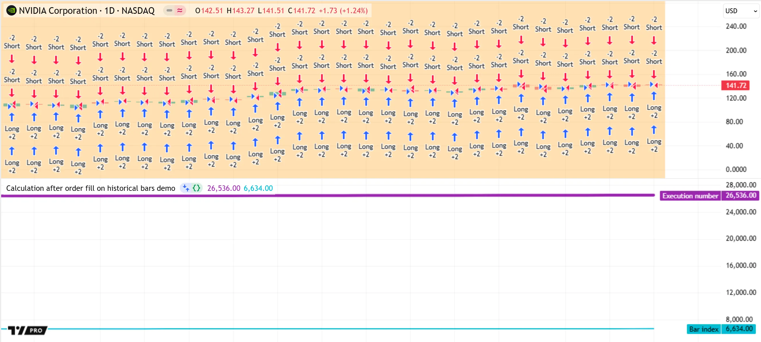
Note that:

• This script can execute more than four times per bar if it uses Bar Magnifier mode, because this mode enables the broker emulator to fill orders on historical bars using intrabar prices from a lower timeframe.
• The script can execute numerous times on a realtime bar, depending on the updates from the data feed, because each new update to the bar is a valid tick for filling the strategy’s orders.
• An alternative way to confirm the script’s increased execution count is to select and clear the “After order is filled” checkbox in the “Settings/Properties” tab while profiling the code.

Executions on realtime bars

After a script running on the chart or in an alert executes across all historical bars in a dataset, the runtime system continues to execute the script on the current bar, if it is open, and on any new bars that form later. We refer to these bars as realtime bars, because they represent incoming data from a separate data feed that the script can access only after it finishes loading.

As explained in the previous section, historical bars represent confirmed data points. By contrast, a realtime bar represents an initially unconfirmed data point that evolves as new updates (ticks) arrive from the realtime data feed. With each new tick, the bar’s high, low, close, volume, and other values update to represent the latest data while the bar remains open. After the bar closes, it becomes an elapsed realtime bar, whose values no longer change. Then, a new realtime bar opens after another tick arrives, and that bar updates as new data becomes available.

As an indicator or library script runs on an open realtime bar, its compiled code executes once after every new update from the data feed. With each new execution, the script recalculates its results for that bar using the latest data. Consequently, the states of the script’s variables, expressions, and objects can change with each new execution while the bar remains open. The system commits the script’s data for the realtime bar only after the bar closes.

After each script execution that occurs before a bar’s closing tick, the runtime engine executes a rollback process. Rollback resets applicable script data to the latest committed states in the time series. This process enables the script to recalculate the bar’s results using only the latest available data — without the influence of temporary data from executions on the bar’s previous ticks.

Below, we explain how recalculation and rollback affect a script’s data and outputs, along with some notable exceptions to this process:

Reinitialize variables

The runtime system erases the states of any variables that the script initializes during its executions before a bar’s close, excluding those declared using the varip keyword. When the script executes again after rollback, it reinitializes the variables with new values or references based on the latest available data.

Likewise, the system does not preserve the temporary states of built-in variables that hold values for the current bar. Before the new script execution, it sets the variables to use the bar’s most recent data. For instance, the system updates close, high, and low with the latest, highest, and lowest prices reported since the bar’s opening time.

Reset changes to var variables

Variables that use the var keyword in their declaration are initialized only once — during the first execution of their scopes on a closed bar. Variables that use the var keyword in their declaration remain initialized after the first time that their scopes execute on a bar’s closing tick. Their assigned values or references persist across subsequent bars, changing only after reassignment or compound assignment operations.

Although these variables preserve data across successive bars, they do not preserve data across executions on the ticks of an open bar. Rollback reverts all variables declared with var before the current bar to the last committed states in the time series as of the previous bar.

For instance, if a variable declared with var has a value of 20 on the open bar and 19 on the previous bar, the variable’s value reverts to 19 before the script executes on the next tick of the same bar. The temporary value of 20 does not persist.

Replace plotted outputs

The plot*(), bgcolor(), barcolor(), and fill() functions create visual outputs on every bar. These outputs are temporary on the open realtime bar. When the script executes again after rollback, the new outputs for the bar from calls to these functions replace the ones from the previous tick.

For example, when the expression plot(close) executes on the open bar, it displays the bar’s latest close value as of the current execution. However, the plotted result is temporary until the bar closes. After rollback, the close variable updates, then the script calls plot() again on the next execution to replace the output from the previous tick and display the new value.

Remove and revert objects

User-defined types (UDTs) and special types such as collections and drawing types are reference types. They define structures from which scripts create objects — independent entities that store data elsewhere in memory. Variables of these types hold references that provide access to specific objects and their data; the variables do not store objects directly.

If a script creates objects on an open bar and does not assign their references to variables declared with the varip keyword, the rollback process removes those objects. During the next execution on the open bar, the script creates new objects if the updated logic allows it.

For example, if a script calls label.new() to create a label object on the open bar, the system deletes that object during rollback. On the next execution, the script evaluates label.new() again, creating a new label that replaces the output. The label created on the previous tick no longer exists.

Similarly, for objects of built-in or user-defined types with references assigned to var variables, the rollback process reverts any changes to those objects that occur on the open bar. The only exception is for UDTs with fields that include the varip keyword. See the Objects page for more information.

Exceptions

The runtime system does not revert all the data from script executions on an open bar. The following are notable exceptions to the rollback process:

• Variables or fields declared with the varip keyword do not revert to a previously committed state. They persist across all script executions after initialization, even those on the ticks of an open realtime bar.
• Logged messages in the Pine Logs pane do not disappear after rollback. The messages from any log.*() calls during executions on the ticks of realtime bars remain in the pane until the script reloads.
• The data from strategy orders placed or filled on the ticks within a bar is not subject to rollback. If a strategy script creates orders or the broker emulator fills orders on an open bar, the data from those events persists.
• Rollback does not erase logs for alerts from the “Alerts” menu. All messages from a script alert remain visible until the user restarts the alert.
• Runtime errors from the system or the runtime.error() function completely stop script executions. If an error occurs at any point while a script executes on an open bar, the system halts the script and does not revert the error after new updates from the data feed.

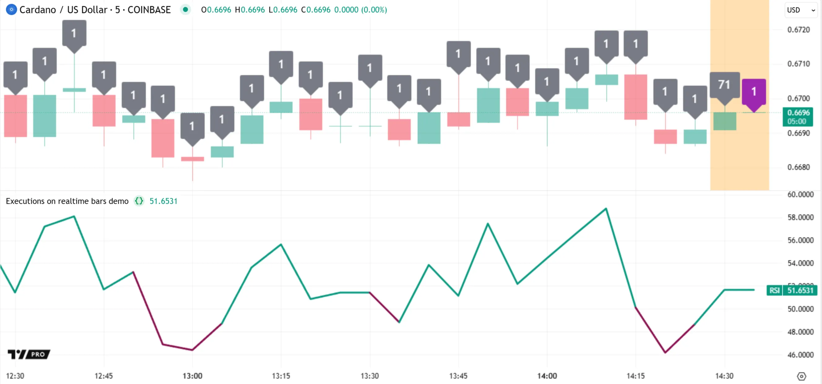
Let’s inspect the behavior of a simple indicator on realtime bars. The following script calculates an RSI of close values using ta.rsi() and displays the result with a plot() call. To track the number of executions that occur per bar, the script increments an executions variable declared with varip and calculates its one-bar change using ta.change(). The script converts each bar’s execution count to a string with str.tostring(), then displays the result in a color-coded label at the bar’s high. The label is purple if the bar is open. Otherwise, it is gray. The script also highlights the background of realtime bars in orange using bgcolor():

When we first add the script to the chart, it does not add an orange background to any bar because it calculates only on data that exists at the script’s loading time. This data is historical. Each bar’s label shows a value of 1 because indicators always execute once per historical bar:

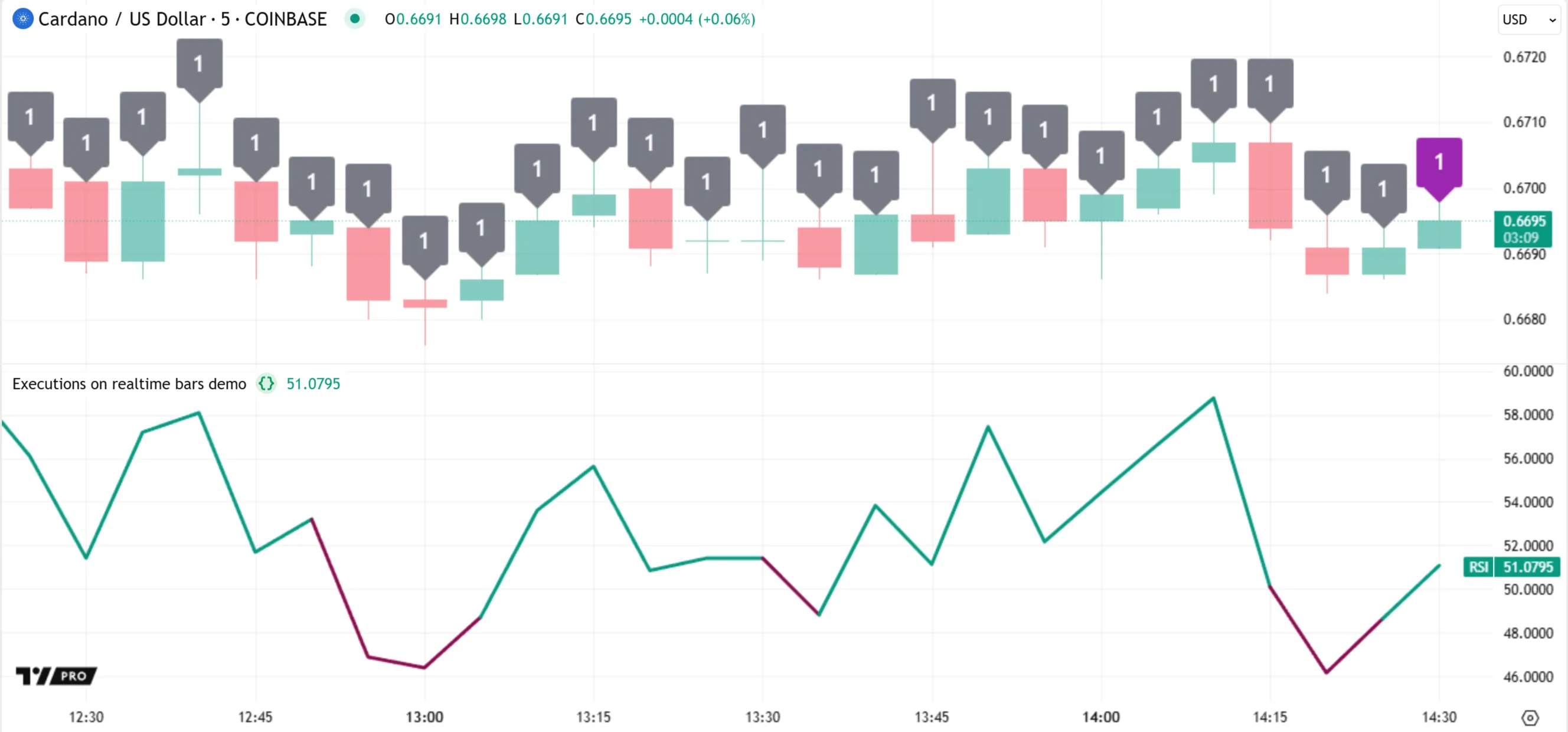
Notice the countdown timer and the purple label for the latest bar in the chart above. These both indicate that the bar is open and subject to changes. A new update from the data feed affects the bar’s values, triggering rollback and a new script execution to recalculate the results.

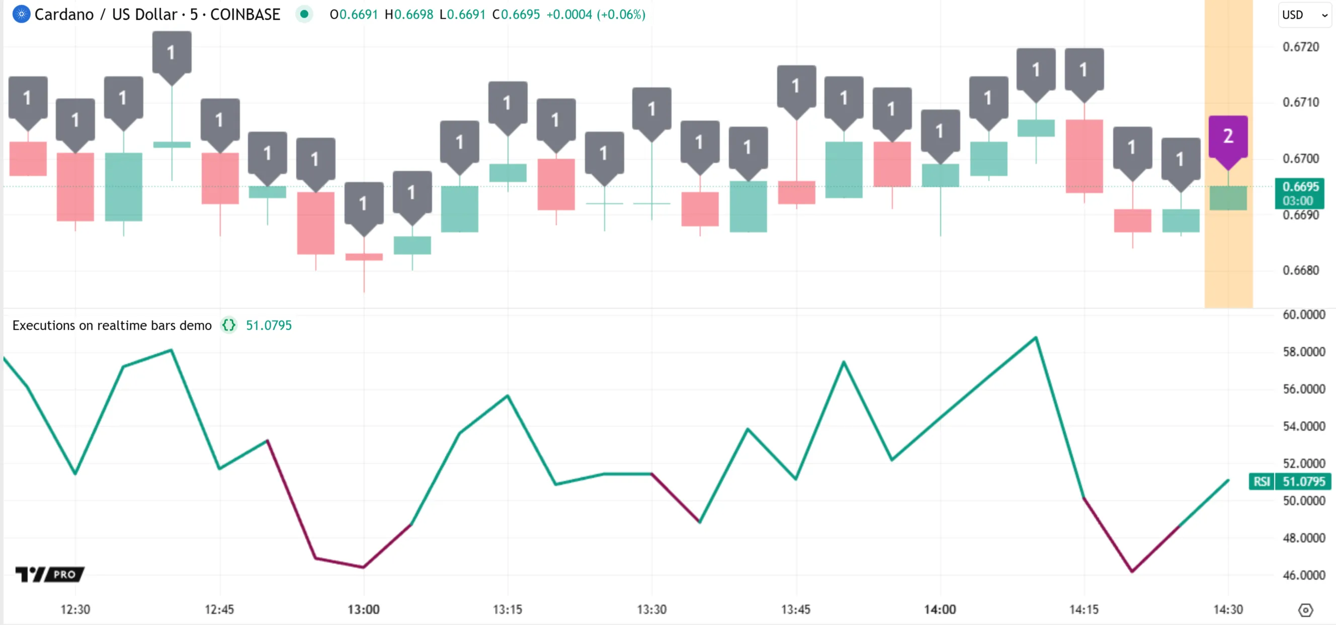
When rollback occurs, the runtime system reverts the internal data of the ta.rsi() call to its last committed state, erases the state of the rsi variable, and deletes the latest label object. However, the system does not revert the executions variable because it uses the varip keyword.

After rollback, the system updates the built-in close, high, and barstate.* variables using the current bar’s latest data, and the new execution begins. The script evaluates the ta.rsi() call using the new close price and reinitializes the rsi variable with the returned value. Then, it increases the executions value by one, evaluates ta.change() again, and creates a new label at the bar’s current high price to show the updated result. Lastly, it evaluates the plot() and bgcolor() calls to replace the bar’s plotted visuals. The last bar’s label remains purple because the bar is still open, but the background color is now orange because barstate.isrealtime is true:

As subsequent updates become available from the data feed, the pattern of rollback and re-execution continues, and the script’s outputs for the bar update with each new execution:

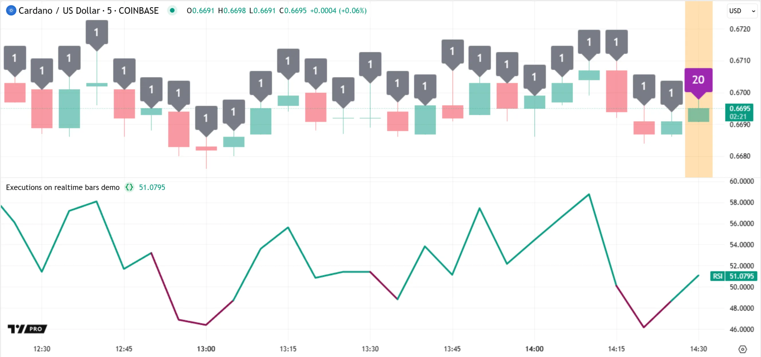
The last time that rollback and another execution occur on this bar is after the closing tick, when the bar becomes an elapsed realtime bar. After the final execution, the bar’s label is gray because barstate.isconfirmed is true. The runtime system then commits necessary data from this execution to the time series for calculations on future bars.

Then, a new realtime bar opens after another update from the data feed, and the execution pattern continues:

Note that:

• Although the previous bar is now confirmed, it still has an orange background corresponding to a realtime state because it closed after the script’s loading time. When the script later reloads after an execution-triggering event, that bar becomes historical.

It’s important to note that strategies often execute differently than indicators on realtime bars. By default, they execute only once per bar at each closing tick without undergoing rollback. However, users can modify a strategy’s calculation behavior to allow rollback and re-execution on a bar before its closing tick.

If the strategy() statement includes calc_on_every_tick = true, or if the user selects the “On every tick” checkbox in the “Settings/Properties” tab, the script executes on a realtime bar after each new update from the data feed, similar to an indicator.

Additionally, if the strategy() statement includes calc_on_order_fills = true or the user selects “After order is filled” in the “Settings/Properties” tab, the script executes on each tick where the broker emulator fills an order. With this behavior, the system can execute the script multiple times on the open bar, but only on the ticks where an order fill occurs.

To summarize the general process for script executions on realtime bars:

• An indicator or library script executes on the first available tick in an open realtime bar, then once per update to recalculate the results for the bar using the latest data. A strategy script executes only on the bar’s closing tick by default, but users can modify its calculation behavior to allow executions while the bar is open.
• Before each new script execution on an open bar, the runtime system executes a rollback process, which reverts all applicable variables, expressions, and objects to their last committed states as of the previous bar’s close.
• After the script executes on an elapsed realtime bar’s closing tick, the system commits necessary data from that execution to the time series for access on later bars. It does not commit the data from executions on the bar’s unconfirmed values from previous ticks.

Events that trigger script executions

Several events cause a script to load and execute across all the available bars in a dataset. The specific events that trigger the loading process depend on where the script runs.

For a script on the chart, the following events always cause the script to load and perform new executions on every bar:

• The user adds the script to the chart for the first time from the Pine Editor or the “Indicators, metrics, and strategies” menu.
• The user saves an update to the script while it is active on the chart.
• The chart is refreshed while the script is active.

Other events also trigger the loading process for a script on the chart. However, these events do not always cause new script executions on past bars. The results from running a script with a unique combination of settings are often temporarily cached. If cached data exists for a selected combination of settings, the system loads the script using that data. See the Caching section for more information.

Below are the additional events that cause a script to load on the chart, either by performing new executions across the dataset or by using available cached data:

• The user selects new values for the inputs or strategy properties in the script’s “Settings” menu.
• The script uses the chart.left_visible_bar_time or chart.right_visible_bar_time variable, and the visible chart range changes.
• The script uses the chart.fg_color or chart.bg_color variable, and the user changes the chart’s background color.
• The chart loads a new dataset with a different timeframe or ticker identifier. Several user actions affect a chart’s ticker ID, such as selecting a symbol from the “Symbol Search” menu, changing the chart type, toggling data modifications in the chart’s settings, and activating Bar Replay mode.
• The user opens or closes the Pine Logs pane.
• The user activates or deactivates the Pine Profiler.

For scripts used in other locations, the following events trigger the loading process:

• The user creates a new script alert from the “Create Alert” dialog box.
• The user pauses and restarts an alert instance from the “Alerts” menu.
• The user clicks the “Generate report” button in the Strategy Tester while Deep Backtesting mode is enabled.
• The user clicks the “Scan” button in the Pine Screener to run the script on the datasets from a chosen watchlist.

After a script loads, either of the following causes new script executions on an open bar:

• One of the events above causes the script to load again and execute across the entire dataset up to the bar.
• The script runs on the chart or in an alert, and the bar updates after new data becomes available. The system performs rollback and re-executes the script on that bar using the latest data. The only exception is if the script is a strategy that does not allow recalculation on the new tick.

When a script completely reloads on the chart or in an alert after an applicable event, all the elapsed realtime bars from the script’s previous run become historical bars in the new run, because they represent confirmed data points that the script accesses from a different data feed as it loads.

The bars in a symbol’s dataset come from two distinct data feeds: the historical feed and the realtime feed. The historical feed reports only the final values for each bar, whereas the realtime feed includes the temporary values from all available ticks. When a realtime bar becomes historical after a script restarts, the values from the bar’s previous ticks are no longer accessible; only the final price, volume, and other values remain. Therefore, if a script relies on temporary data from realtime bars in its calculations, it might behave differently after reloading.

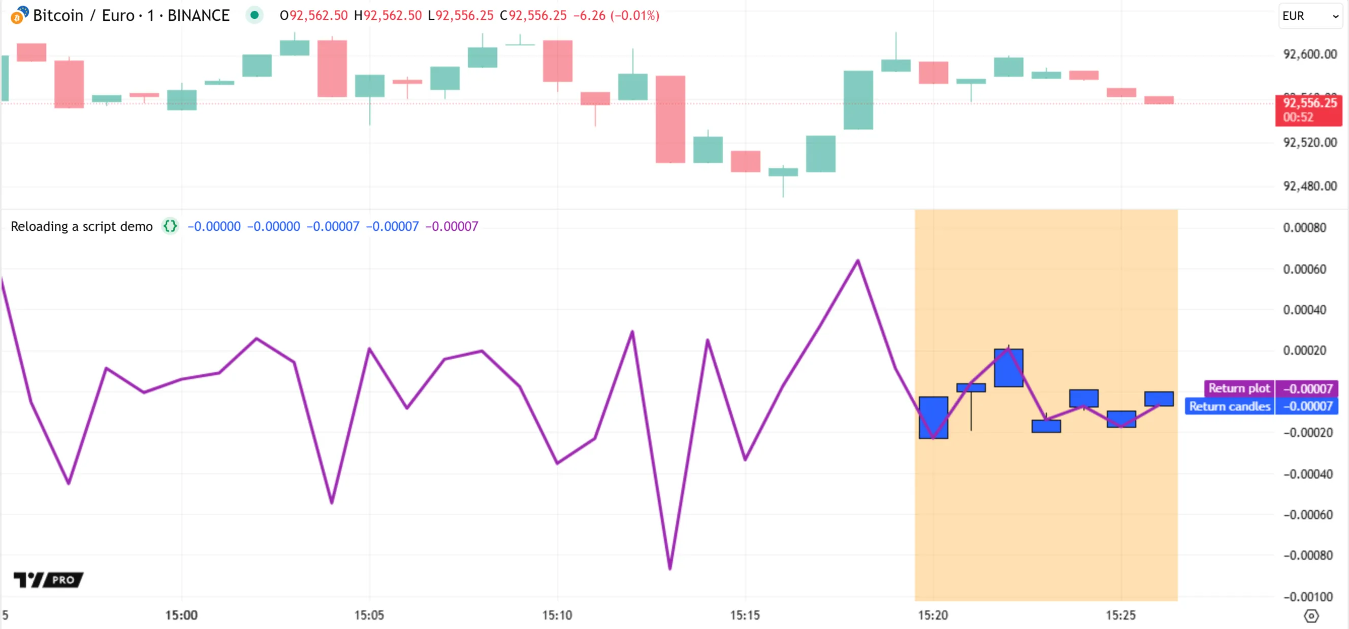
For example, the following script calculates the one-bar arithmetic return of the close series and displays the result as a line plot. On each realtime bar, the script updates three variables declared with varip to track the first, highest, and lowest return values calculated during executions across the bar’s ticks, then calls plotcandle() to plot a candle showing the values. Additionally, it uses bgcolor() to highlight the background of realtime bars in orange:

After the script loads on the chart and executes on several realtime bars, all the elapsed realtime bars, as well as the open realtime bar, include plotted return candles and an orange background color:

After an applicable event, such as a chart refresh, the script reloads and executes across the dataset again. All the closed bars with a realtime state in the previous run become historical bars in the new run. The results thus change because our script relies on realtime data. As shown below, the script does not display candles or background colors for previous bars after we refresh the chart. Those outputs appear only for the latest bar, after new ticks become available, because that bar is now the only one with a realtime state:

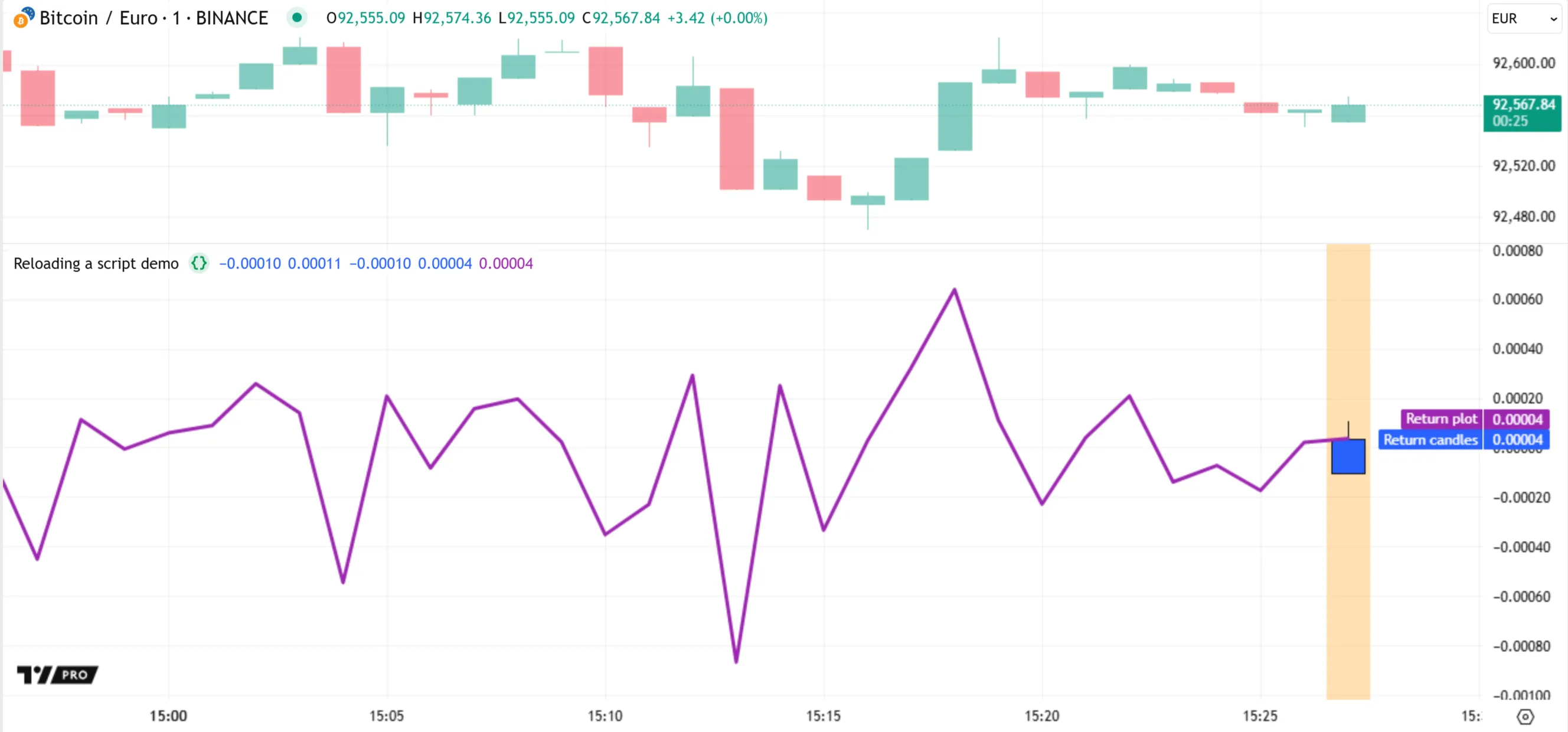
Note that:

• The barstate.isnew variable has a value of true when a realtime bar opens, and false on all subsequent updates to the bar. If the script reloads midway through a realtime bar’s progression, only the background color appears on that bar. The script does not show a candle on the first realtime bar in that case, because its o, h, and l variables hold na until the first time that barstate.isnew is true.

Caching

When a script runs on a chart for the first time using a unique configuration, the data from that run is often temporarily cached for reuse. The cached data is erased after the chart is refreshed or the user updates the script’s source code.

In this context, the configuration refers to the combined state of all script, chart, and developer tool settings that can affect the script’s executions. This combination includes:

• The values of inputs in the script’s “Settings/Inputs” tab.
• The values of the strategy properties in the “Settings/Properties” tab.
• The values of the chart.* variables whose qualifiers are “input” (chart.left_visible_bar_time, chart.right_visible_bar_time, chart.fg_color, and chart.bg_color).
• The chart’s timeframe.
• The chart’s ticker identifier.
• Whether the Pine Logs pane is open or closed.
• Whether the Pine Profiler is active or not.

Each time that a script runs using a unique combination of settings, it executes from start to end on each bar in the dataset to perform new calculations. If possible, the script’s data from the run is then cached. If cached data is available on past bars for a selected combination of settings, the runtime system loads the script using that data.

This behavior enables users to change a script’s inputs, alter the chart, and toggle developer tools without losing information — including bar states — from previous script runs using different settings. Additionally, caching helps reduce loading times and resource requirements when switching between settings or adding multiple instances of the same script to the chart.

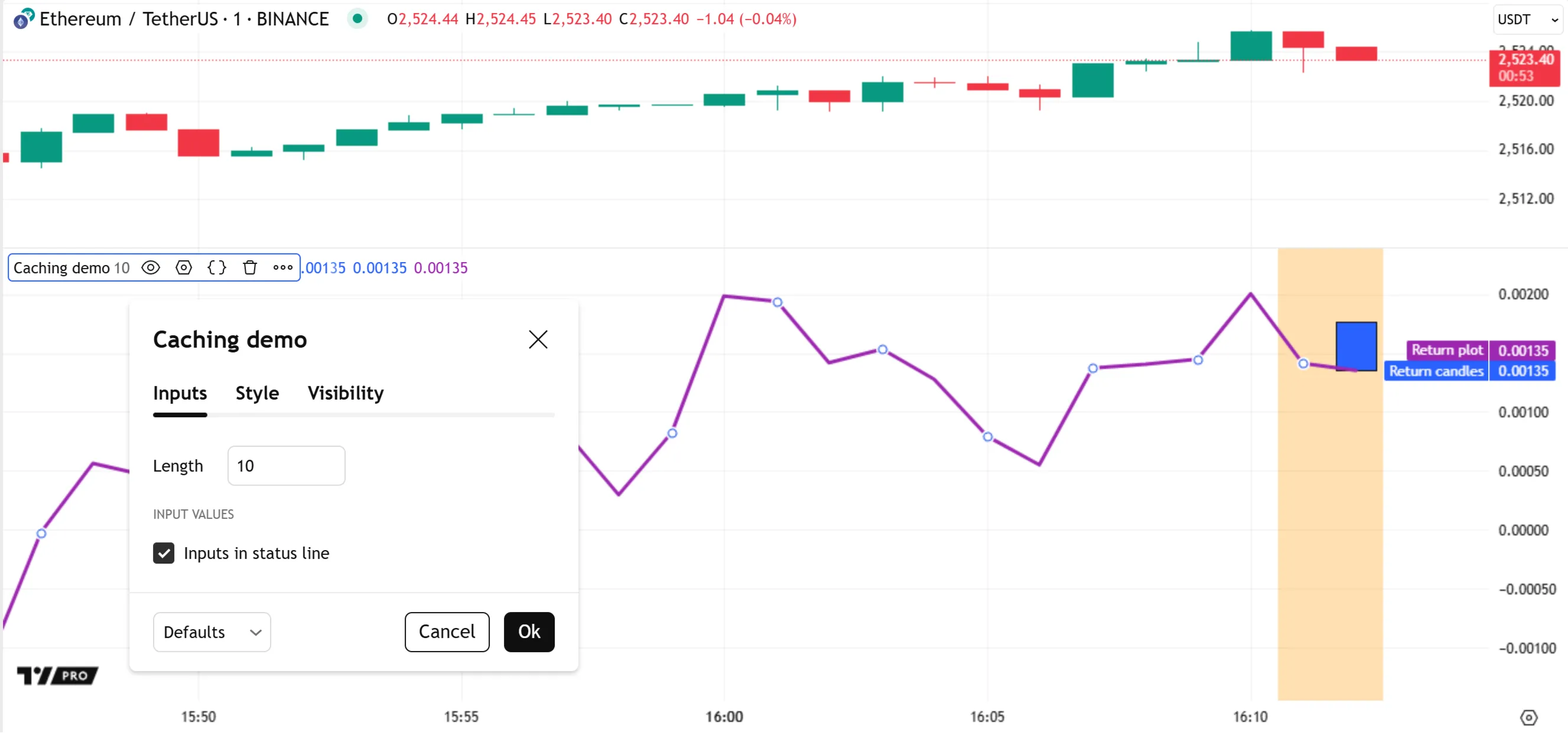
To understand this behavior, let’s revisit the script from the previous section. The script has different behaviors on historical and realtime bars. In the version below, we’ve added a lengthInput variable that holds the value from an input.int() call. The script uses this variable to define the length of the ta.change() calculation and the offset of the history-referencing operator:

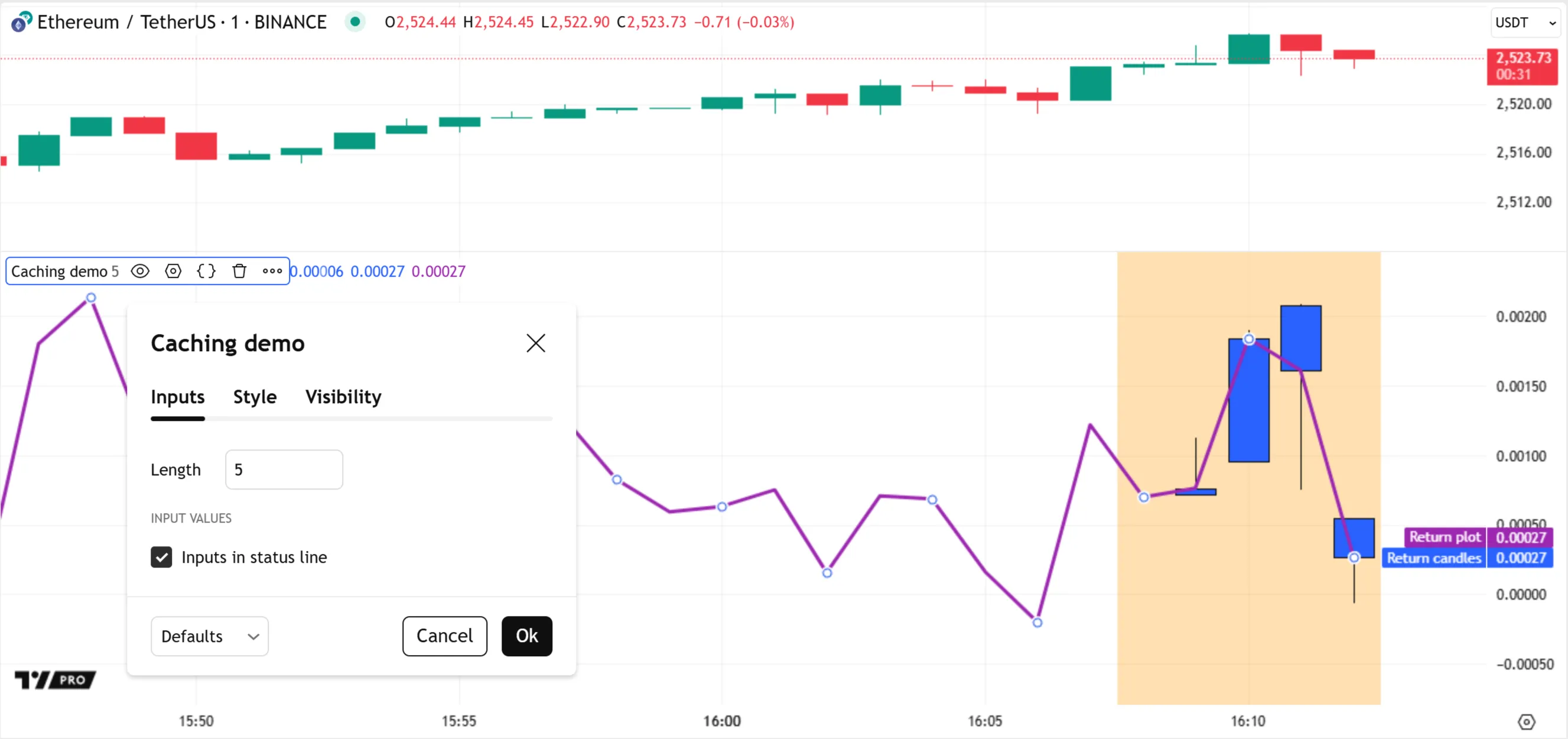
After we add the script to our 1m chart and let it run for a few minutes with a “Length” input value of 5, the script plots candles and highlights the background for the latest few bars, because barstate.isrealtime is true on those bars:

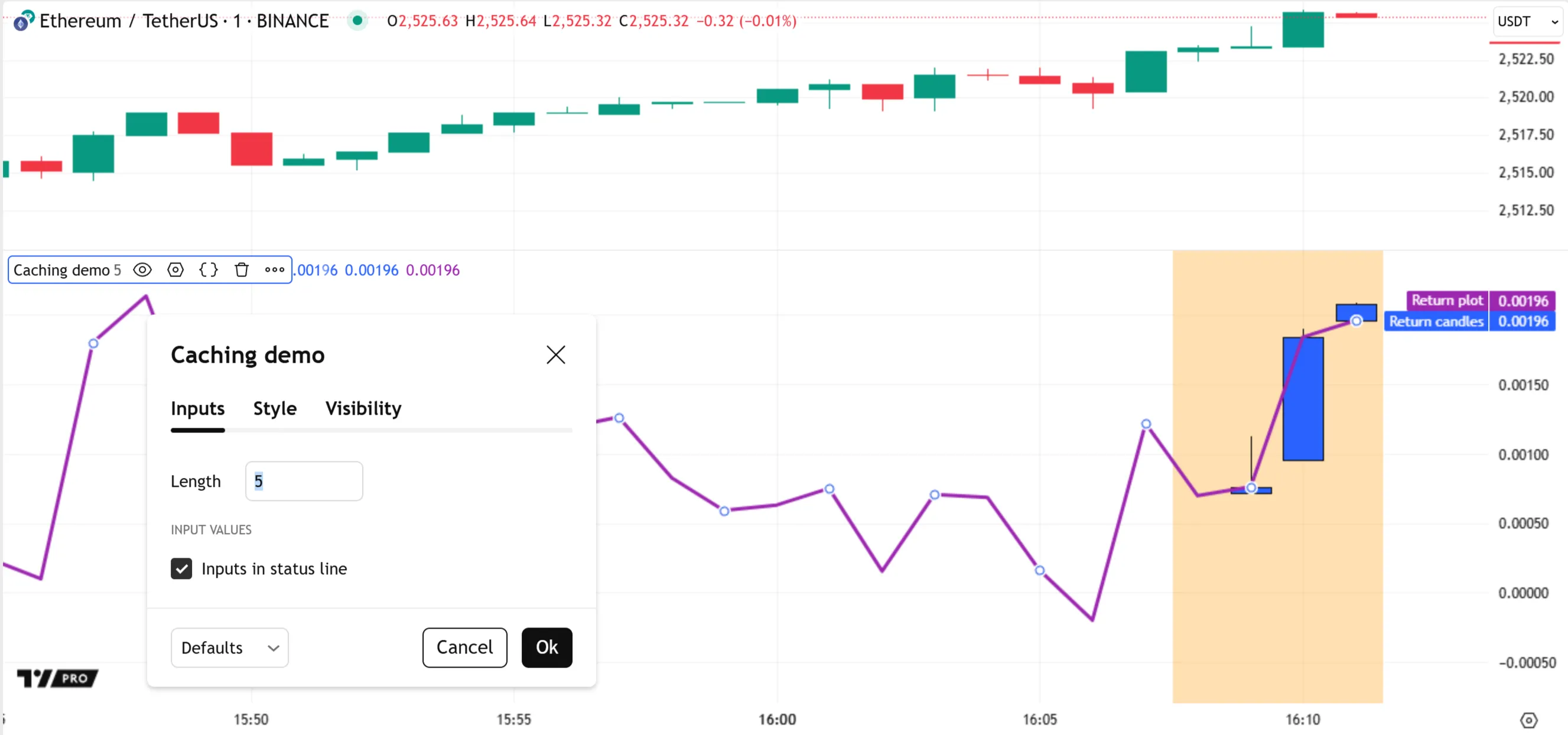
Let’s change the “Length” input to a new value, causing the script to reload and execute across the dataset again. Here, we changed the value from 5 to 10 and let the script execute on some new ticks. The script no longer displays candles and background colors for the same bars after restarting, because it now accesses the data for those formerly realtime bars from the historical data feed:

As shown above, the realtime bar information from the first run is not available when we change the script’s input to a new value. However, the data from that previous run still exists in memory. If we revert the “Length” input’s value to 5, the candle plot and background colors start on the same bar as the first run:

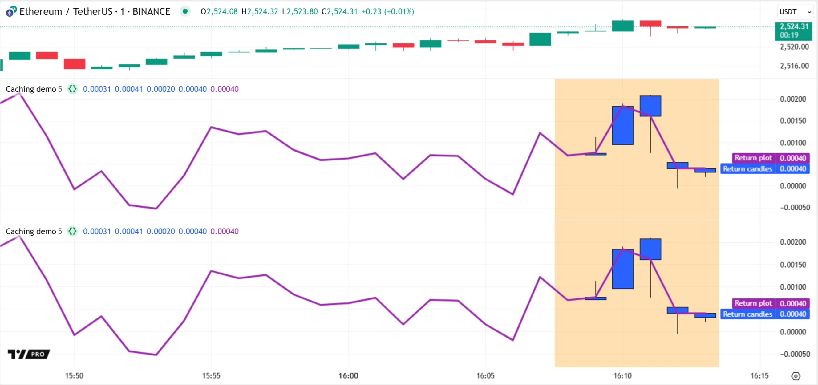
If we add a second instance of the script to the chart, using the same settings, the runtime system loads the new instance using the cached data instead of executing it entirely from scratch. As such, its outputs are identical to those from the first script instance, even though we added it to the chart a few bars later:

Similarly, cached data usually remains available even if we remove the script from our chart and add it again.

Time series

A symbol’s dataset is a form of time series — a sequence of collected values indexed by time. Each bar represents a distinct data point, anchored to a specific time, that contains price and volume data for a particular period. This data format thus shows how a symbol’s values progress across time in successive periodic steps.

Pine Script’s internal time series structure follows a similar format. After executing a script on a closed bar’s confirmed values, the runtime system commits (saves) the results of the script’s statements and expressions to internal time series for later use. Each bar with committed data has an assigned index in the series, where 0 represents the first bar, 1 represents the second, and so on. Scripts can retrieve this index with the bar_index variable.

Scripts can access the data committed to the time series on past bars by using the [] history-referencing operator. The value between the operator’s square brackets specifies the position of the referenced bar in the time series as a relative offset behind the current bar. For variables and expressions in the global scope, an offset value of 1 refers to the previous bar at bar_index - 1 (one bar back), a value of 2 refers to the bar at bar_index - 2 (two bars back), and so on. An offset of 0 always refers to the current bar.

For example, consider the open variable, which holds the opening price of the current bar on which the script executes. Before each script execution on a new bar, the runtime system commits the open value from the last execution on the previous bar. Then, it updates the variable to hold the current bar’s opening price. To access the committed open value for the previous bar, we can use the expression open[1]. To access the committed value from 10 bars back, we use open[10].

The script below performs three history-referencing operations to retrieve the current bar’s open value, the value from one bar back, and the value from a user-specified number of bars back. Then, it plots the retrieved values on the chart for comparison:

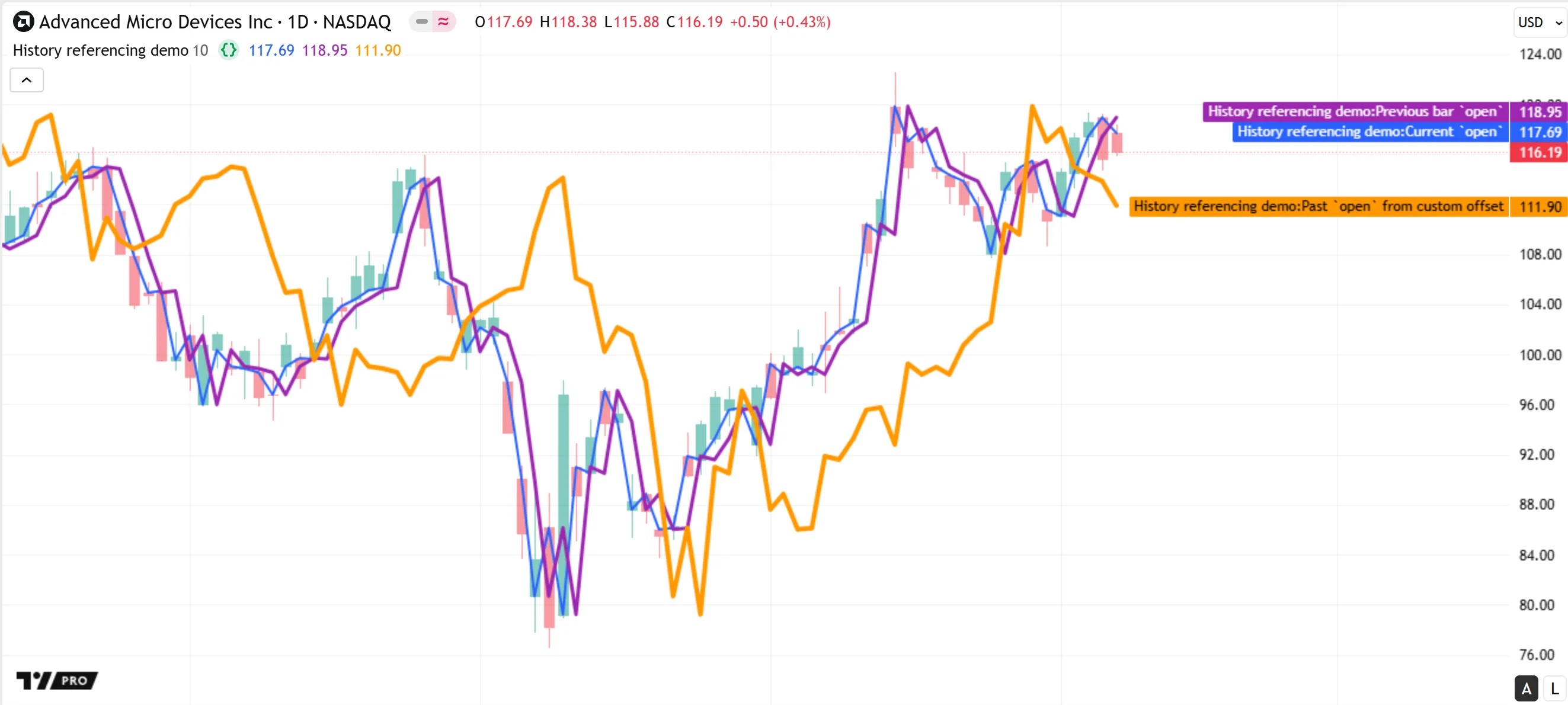
Note that:

• The expression open[0] is equivalent to using open without the history-referencing operator, because an offset of 0 refers to the current bar.
• At the beginning of the chart’s dataset, the expressions open[1] and open[offsetInput] return na because they refer to previous bars that are unavailable.
• Each history-referencing expression also leaves a trail of values in the time series. Therefore, it is possible to retrieve past states of the expression using another history-referencing operation, e.g., (open[offsetInput])[1].
• Internally, the system maintains a limited amount of time series data for variables and expressions in fixed-length historical buffers. These buffers define the maximum offsets allowed for history-referencing operations. See the next section, Historical buffers, to learn more.

Another way that scripts use committed values from a time series is by calling the built-in functions that reference history internally, such as those in the ta.* namespace. For example, the expression ta.highest(high, 20) calculates the highest value from the high series over a 20-bar window. It compares the series’ current value to the committed values from the previous 19 bars to determine the result. The script below executes this call on each bar and plots the resulting series on the chart. Additionally, the script colors the background of the last 20 bars on the chart to highlight the bars used in the latest execution’s ta.highest() call:

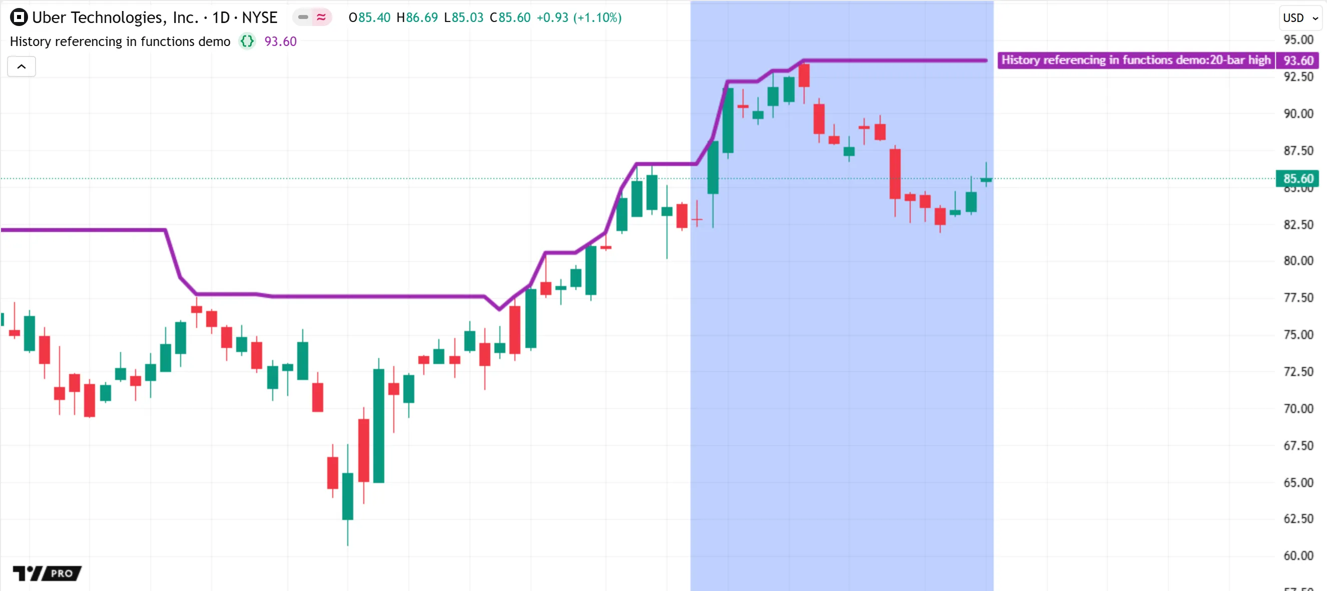
Note that:

• The first 19 bars of the chart have a plotted value of na, because the ta.highest() function call requires the high values from the current bar and 19 previous bars to calculate the result.
• All function calls and expressions that do not return “void” leave historical trails in the time series, just like variables. Therefore, scripts can use an expression such as ta.highest(high, 20)[10] to retrieve the 20-bar high from 10 bars back.
• The ta.highest() function and other functions that access past values from a time series must execute in the global scope for consistent calculations. Time series storage for variables and expressions in local scopes works differently than that for global values. See the Time series in scopes section for more information.

Historical buffers

To promote efficiency and help ensure computing resources remain available for all users, the Pine Script runtime system uses fixed-length historical buffers to maintain a limited amount of time series data for all variables and expressions. These historical buffers define the maximum number of committed data points that a script can access on any bar via the history-referencing operator or the built-in functions that reference past bars internally.

For most series, the underlying historical buffer can contain data from up to 5000 past bars. The only exception is for some built-in series such as open, close, and time, whose buffers can store data for more than 5000 bars.

Although these buffers can contain thousands of data points at their maximum size, a script might not require that much past data for its calculations on any bar. Therefore, the runtime system automatically optimizes the size of each series’ historical buffer based on the historical references that the script performs as it loads on the dataset. Each resulting buffer contains only the amount of past data required by the script’s calculations and not more.

For instance, if the maximum number of bars back for which a script references the value of a variable on historical bars is 500, the system maintains a historical buffer that includes only the latest 500 committed values of that variable. The buffer does not store 5000 committed values, because the script does not require all that extra data. This behavior thus helps to minimize a script’s resource requirements while preserving the integrity of its calculations.

To determine the sufficient buffer size for each variable and expression in a script, the runtime system performs the following process during the script’s loading time:

1. It analyzes all the historical references that occur while executing the script on the dataset’s first 244 bars, then sets the initial size of each buffer to the minimum size that accommodates those references.
2. While executing the script on subsequent bars, it checks if the script attempts to access data from previous bars that are beyond the limits of the defined buffers. If the script’s historical references exceed the buffer limits on any bar, the system restarts the loading process and tries a larger buffer size.
3. In the rare case that a historical buffer’s size remains insufficient after several calculation attempts, the system stops the script and raises a runtime error.

It’s crucial to emphasize that the runtime system defines the sizes of all historical buffers only while executing a script on historical bars. It does not adjust any historical buffers during executions on new bars from the realtime data feed. If a script references past data from beyond a historical buffer’s limits while executing on a realtime bar, it causes a runtime error.

For example, the script below retrieves a past value from the close series using the history-referencing operator with an offset of 100 bars back on historical bars and 150 bars back on realtime bars. Because the script references data from 100 bars back during all historical executions, the system sets the close buffer’s size to include only 100 past values. Consequently, an error occurs when the script executes on the open realtime bar, because a historical offset of 150 is beyond the buffer’s limit:

For cases like these, programmers can manually set the size of a historical buffer to ensure it contains a sufficient amount of data by doing any of the following:

• Modify the script to reference the maximum required number of bars back with the [] operator during its execution on the first bar.
• Call the max_bars_back() function to explicitly set the historical buffer size for a specific series.
• Include a max_bars_back argument in the indicator() or strategy() declaration statement to set the initial size of all historical buffers.

Below, we modified the script by including the expression max_bars_back(close, 150), which sets the size of the close buffer to include 150 past values. With the appropriate buffer size manually defined, the script’s history-referencing operation no longer causes an error on realtime bars:

Time series in scopes

The scope of a variable or expression refers to the part of the script where it is defined and accessible in the code. Every script has one global scope and zero or more local scopes.

All variables and expressions in a script that are outside user-defined functions or methods, conditional structures, loops, and user-defined type or enum type declarations belong to the global scope. The script evaluates variables and expressions from this scope once for every execution across bars and ticks in the dataset.

All functions, methods, conditional structures, and loops create their own local scopes. The variables and expressions defined within a local scope belong exclusively to that scope. In contrast to the global scope, a script does not always evaluate a local scope once per execution; the script might evaluate the scope zero, one, or several times per execution, depending on its logic.

For the runtime system to commit data from a variable or expression and queue that data into a historical buffer on any bar, a script must evaluate the scope of that variable or expression once when it executes on the bar’s closing tick. If the script does not evaluate the scope, the runtime system cannot update the historical buffer for the variable or expression. Similarly, if the script evaluates the scope repeatedly within a loop, the historical buffer cannot store series data for each separate iteration, because each entry in the time series corresponds to a single bar.

Therefore, time series behave differently in global and local scopes: the historical buffers for global variables and expressions always contain committed data for consecutive past bars, whereas the buffers for local variables often contain an inconsistent history of committed data.

When a script references the history of a global variable using an expression such as myVariable[1], the historical offset of 1 always refers to the confirmed myVariable value from the previous bar. In contrast, when using such an expression with a local variable, the offset of 1 refers to the most recent bar where the script executed the scope. It does not represent a specific number of bars back. Therefore, referencing the history of a local variable can cause unintended results.

The following example demonstrates how the historical buffers for a user-defined function’s local scope behave when a script does not call the function on every bar. The script below contains a custom upDownColor() function, which compares the current value of its source parameter to the last committed value (source[1]). The function returns color.blue if the current source value is higher than the previous value. Otherwise, it returns color.orange.

The script uses this function conditionally, inside a ternary operation, to determine the color of a plot that shows the remainder from dividing bar_index by a specified value. If the remainder variable’s value is nonzero, the operation calls upDownColor(remainder) to calculate the color (blue or orange). If the value is 0, the operation does not use the call and instead returns color.gray. The remainder value increases on each bar, except for when it returns to 0 — causing the gray color. Therefore, a user might expect the plot’s color to be only blue or gray on every bar. However, the color changes to orange on each bar after the one where the color is gray, even though the remainder value on that bar is higher than the value on the previous bar:

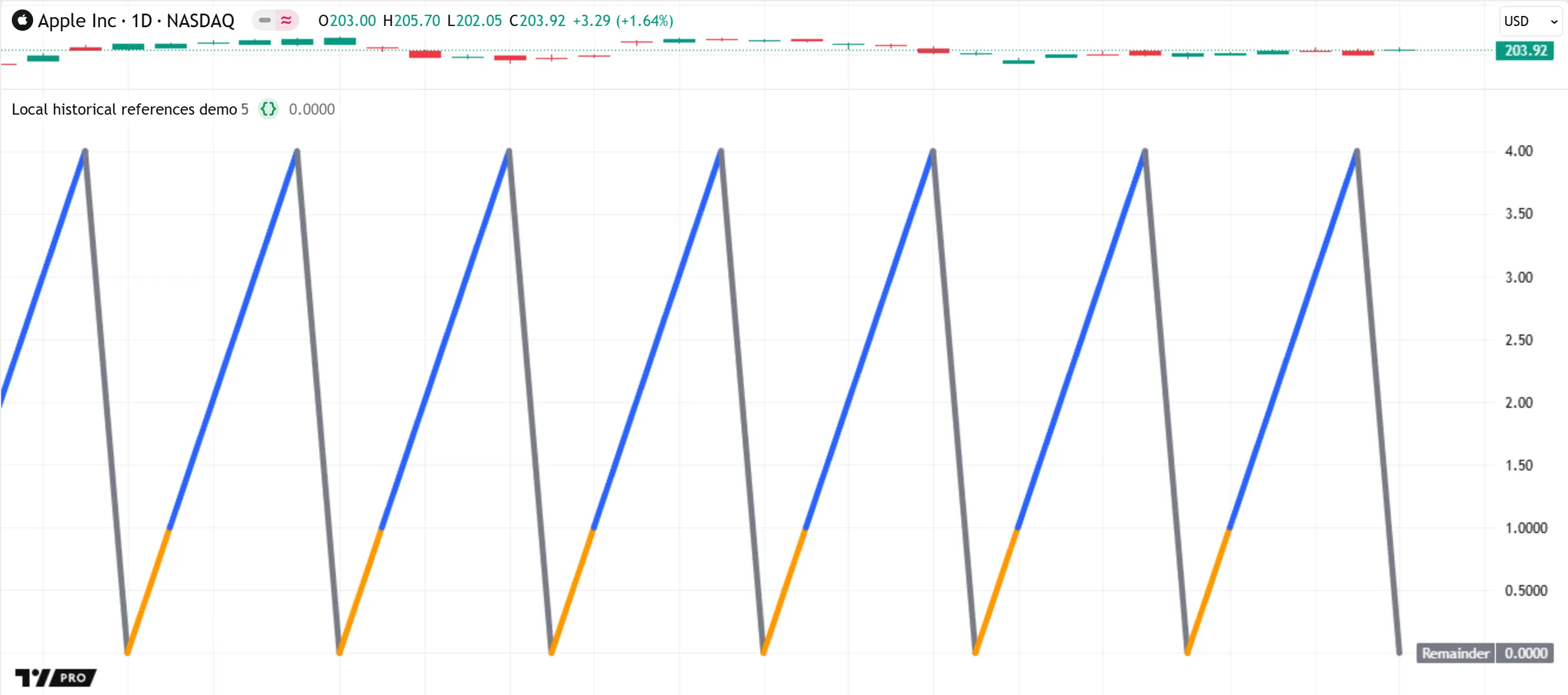
The script behaves this way because upDownColor() uses the history-referencing operator on the source series, which is local to the function’s scope, and the script does not call the function on every execution. When the value of remainder is zero, the first expression in the ternary condition evaluates to true, and therefore the second branch of the ternary expression, which contains the function call, does not execute.

The compiler issues the following warning about the function directly in the Pine Editor:

The function `upDownColor()` should be called on each calculation for consistency. It is recommended to extract the call from the ternary operator or from the scope.

The runtime system maintains a separate historical buffer for the local source series, but it cannot update that buffer unless the script calls the function. On each bar where remainder is 0, the call does not occur, and the system has no new value to commit to the time series. Therefore, the source buffer does not contain the value of remainder, or even an na value, for that bar. On the bar that follows, the local expression source[1] refers to the source value from the last bar where the upDownColor() call occurs — two bars back — and not the value of remainder from the previous bar. Because the value from two bars back is higher than the current value, the returned color is color.orange instead of color.blue.

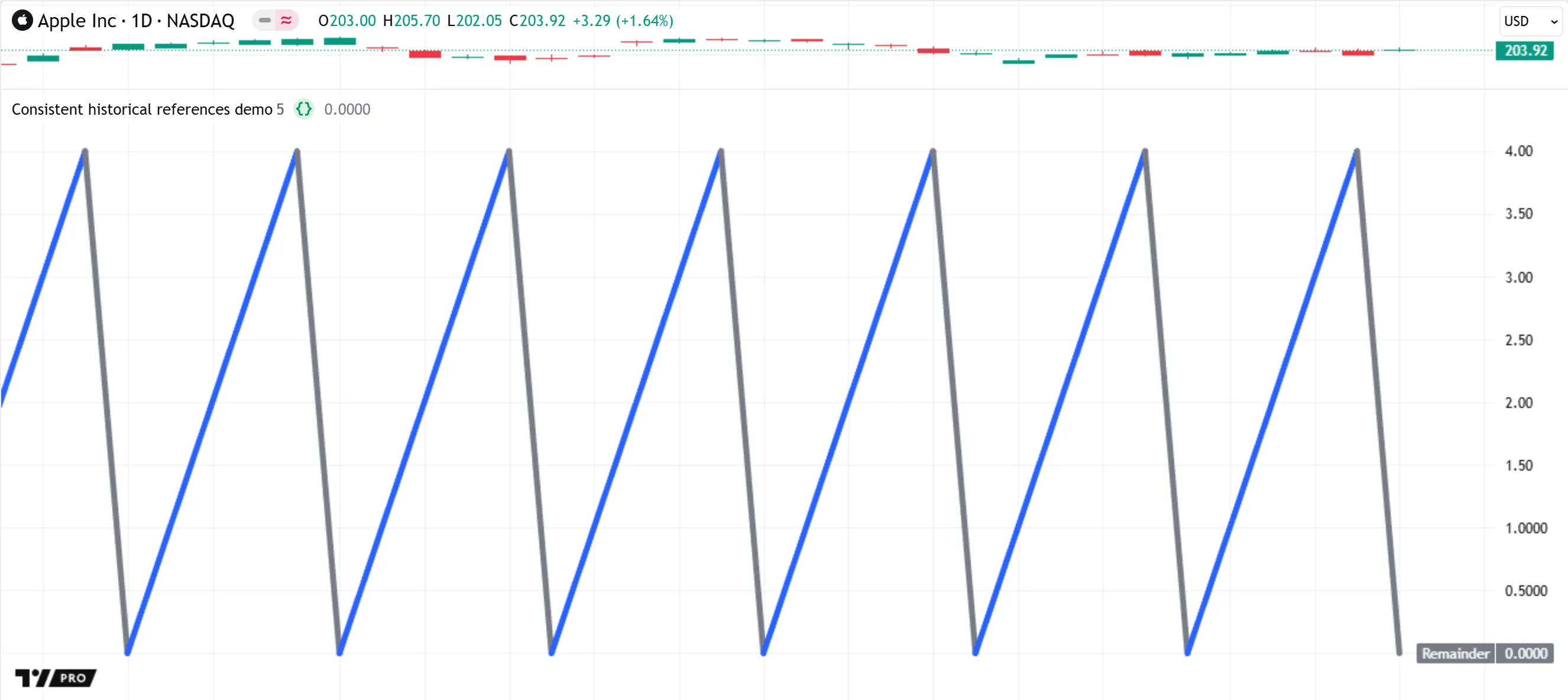
We can fix this script’s behavior by following the instructions in the compiler warning. Below, we modified the script by moving the upDownColor() call outside the ternary expression, enabling the script to execute it on every bar. The historical buffer for the function’s source series now contains remainder values from consecutive bars. With this change, an orange color does not appear because the function consistently compares values from one bar back:

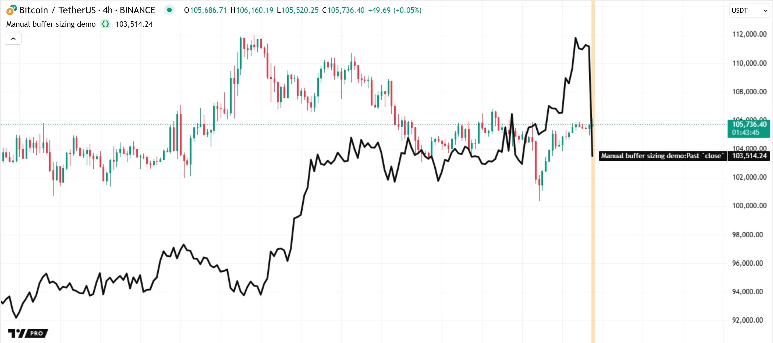
This behavior also applies to all built-in functions that reference past values internally, such as those in the ta.* namespace. For example, the ta.sma() function uses the current value of a source series and length - 1 past values from that series to calculate a moving average. If a script calls this function only on some bars instead of on every bar, the historical buffer for source does not contain values for consecutive past bars. Therefore, such a call can cause unintended results, because the call calculates the returned average using an inconsistent history of values from previous bars.

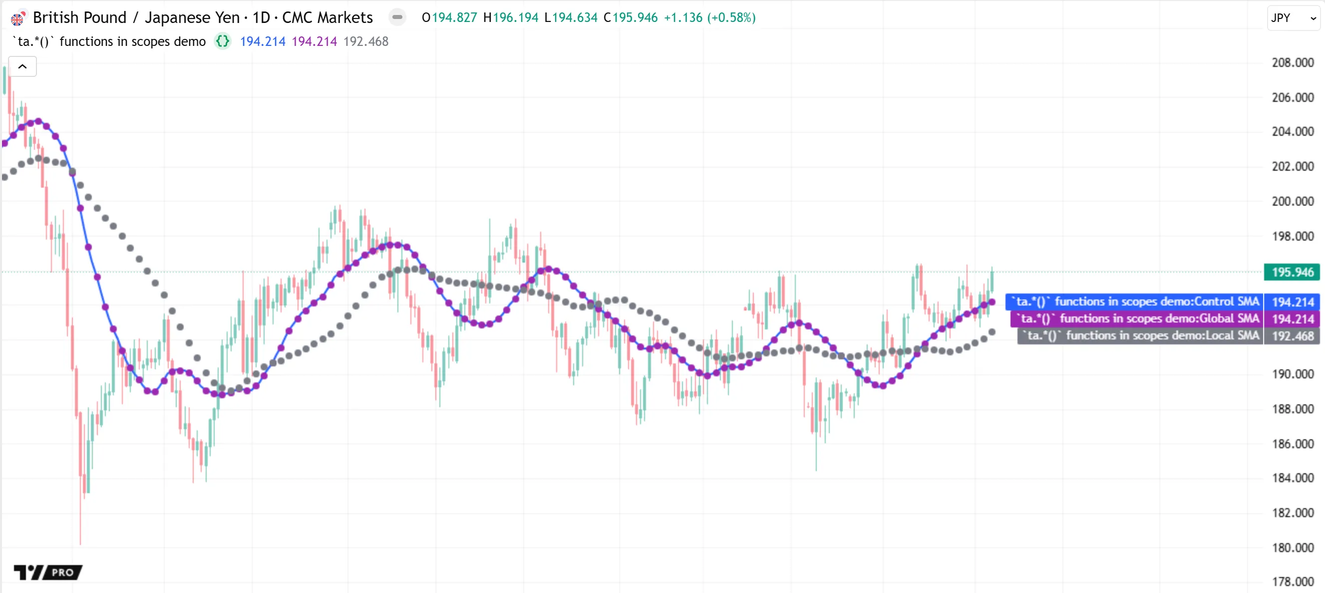
The script below demonstrates how the results of the ta.sma() function can vary with the scope in which the function call occurs. The script declares three global variables to hold calculated SMA values: controlSMA, localSMA, and globalSMA. The script initializes controlSMA using the result of a ta.sma() function call, and it initializes the other two variables with na. Within the if structure, the script updates the value of globalSMA, and it updates localSMA using the result of another ta.sma() call with the same arguments as the first call.

As shown below, the controlSMA and globalSMA have the same value. Both use the result of the global ta.sma() call, which executes on every bar. The internal historical buffer for source in that call thus includes committed values for consecutive past bars. In contrast, the localSMA value differs, because the ta.sma() call for that variable does not execute on every bar. The buffer for that call’s local source series contains only the values from bars with an even bar_index value:

To summarize the behavior of time series in a script’s scopes:

• A script evaluates its global scope once on every execution. After each script execution on a bar’s closing tick, the system commits the data for variables and expressions in the global scope and updates their historical buffers. The resulting buffers thus include data for consecutive past bars, ensuring consistent results for operations and functions that rely on past data.
• A script evaluates local scopes zero, one, or several times per execution. The runtime system cannot maintain consistent bar-by-bar historical buffers for scopes that a script does not evaluate on every bar, or for scopes that the script evaluates more than once on a bar’s closing tick. Therefore, using the [] operator on local variables and expressions, or not calling functions that access past data once on each closing tick, can cause unintended results.